- +1
- BU
- KK
- PM
776
167
0
Field
Economics, Econometrics and Finance
Subfield
Economics and Econometrics
Economic Evaluation of Ewanrigg Botanical Gardens in Zimbabwe Using an Individual Travel Cost Approach
Precious Mahlatini1, Kudakwashe Bryan Kusuwo1, Beaven Utete2![]() , Nobert Tafadzwa Mukomberanwa3
, Nobert Tafadzwa Mukomberanwa3
Affiliations

Abstract
Economists face an environmental goods and services valuation dilemma as natural resources are considered to be common pool resources with no markets. If markets exist they are mostly imperfect which results in undervaluation or overvaluation of natural resources. This study estimated the imputed recreational use value of Ewanrigg Botanical Gardens in Zimbabwe from 2015‑2017 using the Individual Travel Cost Method (ITC) which elicits the consumer surplus and deduces an optimum entry fee. It investigated key socioeconomic factors which influence visits to Ewanrigg Botanical Gardens. A questionnaire survey was conducted on 54 visitors to Ewanrigg Botanical Gardens during the period of the research to solicit for primary data. The primary data were analysed using the Ordinary Least Squares model to obtain a predictive model of visits to Ewanrigg Botanical Gardens. Using the ITC Method the total consumer surplus which equates to the recreational use value of Ewanrigg Botanical Gardens was USD19 142.16/peak period/year. Travel costs, income and employment status were the major factors driving visitation rates to Ewanrigg Botanical Gardens at an optimum entry fee of USD7.81. To maximise profits for self-sustenance of Ewanrigg Botanical Gardens, the Zimbabwe Parks and Wildlife Authority should concentrate on marketing efforts to individuals of higher income and solid employment status and those proximal to the botanical gardens as these incur less travel costs and can afford entry fees. For posterity, the use of ITC Method to ascertain economic value allows for the true valuation of natural resources and is justifiable for the allocation of funds by central government for the management and maintenance of artificial heritage sites such as Ewanrigg Botanical Gardens in developing African countries.
Corresponding author: Beaven Utete, beavenu@gmail.com
Introduction
Botanical or botanic gardens or arboreta are man-made ecosystems focusing on propagation and cultivation of exotic plant species mainly to illustrate the relationships within plant groups for nature preservation, scientific research, recreation and mental and physical well‑being of the public (GoZ, 2014; Carrus et al., 2015; Chen and Sun, 2018). Like forests, aquariums, orchards, to name but just a few, botanical gardens have direct and indirect value uses which substantially contribute to human welfare (Gómez-Baggethun et al., 2010; Mounce et al., 2017). Botanical gardens facilitate protection of various plant communities and raise awareness about biodiversity values and have assumed an importance in the current climate change discourse (Hill & Gale, 2009; Mounce et al., 2017; Ren and Duan, 2017). Thus, botanical gardens play an imperative role in drawing people and plants together (Demir, 2014). Globally, there are an estimated 2500 botanical gardens (Golding et al., 2010) and these gardens assume an annual visitation rate of 300 million per year (Williams et al., 2015). This implies that botanical gardens generate a substantial amount of revenue for national economies and most importantly for their own sustenance and continuity.
Nonetheless, environmental goods and services provisioned by man-made ecosystems such as botanical gardens are classified as common pool resources or public goods, and thus, they cannot be traded in conventional markets (Costanza et al., 2014). This ultimately results in degradation or underutilization of such resources as the allocated entry fee might be too low which results in visitor congestion affecting the regenerative capacity of the gardens (Chacha et al., 2013; Dixon et al., 2013). Economic valuation is an effort to provide the quantitative monetary value of environmental goods and services whether market value is available or not. It is based on the theory that non-market values can be observed indirectly in consumer expenditure, and in prices of marketed goods and services (Dixon et al., 2013). All decisions that involve trade-offs involve valuation, either implicitly or explicitly (Costanza et al., 2014).
Outdoor recreation such as visiting botanic gardens is undertaken by individuals who anticipate deriving benefit from such. Partially reflected by the entry fee an individual is willing to pay, such benefits can only be comprehensively approximated through non-market valuation techniques such as the Individual Travel Cost Method (Mwebaze & Bennett, 2012) and those indicated in Appendix 1. For this study we used the ITCM Method which evaluates the recreational use value or consumer surplus for a specific recreational site by relating demand for that site (measured as frequency of site visits) to its price (measured as the travel costs) (Safitri, 2018). Hence, Individual Travel Cost Method (ITCM) simply defines the dependent variable as the frequency of visits to a recreational site by each visitor over a defined period as a function of socioeconomic variables inclusive of travel costs (Whitehead et al., 2008; Das, 2013; Limaei et al., 2014)).
Ewanrigg Botanical Gardens measuring 286 hectares is one of the three botanic gardens in Zimbabwe (the others being National and Vumba Botanic Gardens). Due to the garden’s expansive nature, visitors partake in garden viewing (herb garden and water garden), scenic viewing along walking trails, sit and read in the natural serene environment, weddings, barbeque, picnics (GoZ, 2014). Furthermore, the garden is globally renowned for its Cycad and Aloe vera species (Child, 2012). Annually, the garden attracts an average of 248 visitors at an average entry fee of USD3 and USD10 for local and foreign visitors respectively (ZIMPARKS, 2017). However, the entry fee does not reflect the full economic value of the botanical garden due to the informal means of pricing used by the Zimbabwe Parks and Wildlife Authority (Carpenter et al., 2009; Islam & Majumder, 2015). Since the economic value of Ewanrigg Botanical Gardens is unknown, this risks its undervaluation or overvaluation by the Zimbabwe Parks and Wildlife Authority. Moreso, if no formal means are being used for allocating the current price, a question therefore arises on the quantitative magnitude of ecosystem service benefits generated from public access (Bishop & Pagiola, 2012; Demir, 2014).
It is imperative to value botanical gardens as this facilitates determination of optimum entry fees and key socioeconomic factors which influence visits and enhance their maintenance and or further development (Ten Brink, 2012; Paracchini et al., 2014). The main objective of this study was to estimate the imputed economic value of Ewanrigg Botanical Gardens using the Individual Travel Cost Method which elicits consumer surplus and deduce the entry fee. The specific objectives were to i) examine the relationship between socioeconomic factors and number of visits, ii) estimate the economic value of Ewanrigg Botanical Gardens as a recreational site, and iii) estimate the optimum entrance fee to Ewanrigg Botanical Gardens in Zimbabwe.
Study area and Methods
Ewanrigg Botanical Gardens (Figure 1) is located in Shamva District, Zimbabwe. The district lies in the north eastern part of Zimbabwe and shares its boarders with Bindura, and Mt Darwin Districts. It is approximately 35km by road from the capital city Harare. According to ZIMSTATS (2012), Shamva District has a population of 119 530 with 60 099 females and 59 431 males. However, the botanical garden is a very popular recreational site in both Mashonaland Central and Harare Metropolitan provinces. The climate of Shamva District is warm and temperate. In winter, there is little or no rainfall with most precipitation in January. November is the warmest month whilst July experiences the lowest average temperatures annually. The average annual temperature and rainfall for Shamva District is 20.20C and 887mm respectively. Furthermore, irrigation of Ewanrigg Botanical Gardens during dry months is facilitated by the perennial flows of Umfurudzi River.

Data collection and sampling plan
The research collected and analyzed secondary data of the monthly number of visitors to Ewanrigg Botanical Gardens for the period 2015‑2017. A questionnaire (Appendix 2) with both open and close‑ended questions was designed to obtain primary data from visitors to Ewanrigg Botanical Gardens. The former solicited detailed information about visitor attitudes whilst the later solicited information that is easy to statistically analyze. A questionnaire survey was used as it ensures high response rates (Tahzeeda et al., 2018). The questionnaire was designed into two sections:1) personal information on purpose of visit, final visit destination, number of visits per peak period per year, mode/means of transport and place of residence and 2) socioeconomic characteristics of visitors such as age, income, education, gender, marital status and employment status. A survey approach was employed for this study. All visitors to Ewanrigg Botanical Gardens during the study period were surveyed. The average visitation rates were as shown in Figure 2:

High visitor turnouts were observed for May, June, July and August, save for December which is a festive period thus, high visitor turnouts are expected. High visitor turnouts for May, June and July and August were attributed to the full bloom of Aloe vera spp. and Cycad species in winter (Manvitha & Bidya, 2014). Thus, through vernalization, flowering of plants is promoted upon exposure to cold temperatures (Kim et al., 2009). Hence, Ewanrigg Botanical Gardens is always aflame with vibrant colours during this period thereby attracting a considerable number of visitors. High visitor turnouts during the peak visitation period was considered representative of the total annual visits to Ewanrigg Botanical Gardens for this study.
Therefore, an onsite questionnaire survey was conducted from May 1st to July 27th, 2018 between 9am and 5pm on a daily basis. Only visitors over the age of 18years were considered for the survey as the questionnaire included quantitative information such as income and required analytical ability of the respondent (Tahzeeda et al., 2018). Furthermore, the study focused on both frequent foreign (where possible) and local visitors so as to narrow down the research scope and eliminate once off non-traditional visitors to the garden.
Data analysis
Model specification
The ITCM model formulated by (Clawson & Knetsch, 2013) and modified by Twerefou and Ababio (2012); Demir (2014) and Safitri (2018). The demand function of Ewanrigg Botanical Garden (EBG) was formulated as follows:
Vij = f (TCij,Eij,Ai,Ii,Hi,Gi,Mi)| Variable | Explanation |
|---|---|
| Vij | Total number of visits by visitor i to site j (EBG) during the past 12 months. |
| TCij | Round trip travel costs to and fro site j (EBG) incurred by visitor i in $USD |
| Ii | Disposable monthly income of visitor i in $USD |
| Aj | Age of visitor i in years |
| Ei | Visitor i’s years of education |
| Gi | Sex of visitor i, where 1 is Male and 0 is Female. |
| Mi | Visitor i’s marital status |
| Hi | individual i's employment status |
| εij | Unaccounted for variables. |
Total travel costs were a summation of fuel costs and entry fees (ORTAÇEŞME et al., 2002). The fuel cost was USD $1.47 per litre, 11% higher than the global price as of July 27th, 2018. Therefore, assuming fuel consumption rate of 8litres per 100km (ZERA, 2017), the standard fuel cost was calculated as USD$ 0.12 per km, based on the normal fuel costs as of July 27th, 2018.
Relationship between number of visitors and socioeconomic variables
A correlation and linear regression analysis on the number of visits to Ewanrigg Botanical Gardens (dependent variable) against socioeconomic variables of visitors (independent variables) was done. Relative frequencies were also calculated to determine the descriptive statistics pertaining to the socioeconomic variables of the surveyed respondents. From the linear regression model, significant socioeconomic variables that explain the number of visits (Vij) at a significant level of 5% were obtained.
Estimation of the regression model for EBG
A multiple linear regression analysis was performed on the significant socioeconomic variables (from objective 1) against number of visits to obtain a demand function for Ewanrigg Botanical Gardens:
Vij = β0Ai + β1TCij + β2Ii…….+⋯……+εijWhere:
β0, β1, β2, β3- are regression coefficients which measured the changes in the number of visits as a result of a unit change in the socioeconomic variable assuming ceteris paribus.
Calculation of the Individual Consumer Surplus (CS)
The Individual Consumer Surplus was calculated as derived from Equation 2:
Individual Consumer Surplus(CS) = mean V2/-2βTCWhere;
βTC was the coefficient of travel costs from the multiple linear regression analysis of significant variables and V was the total average number of visits by respondents during the past 12 months.
Estimation of the economic value of EBG
The recreational value was obtained by multiplying the individual consumer surplus (CS) by the total number of visitors/peak period/year to Ewanrigg Botanical Gardens as shown below:
Total consumer surplus = CSx total number of visitors peak period / yearDetermination of the optimum entrance fee to EBG
According to the empirical works of Fernando et al. (2016), the number of visits was regressed against the travel costs and a regression equation was obtained as follows;
Vij = β1TCij + intercept (k)By substituting hypothetical entry fees (P) for TCij, a demand curve was obtained relating Vij (Q) and P. The equation was obtained as follows;
P = a – bQHence, when P reached zero, Q was at a maximum and when P was at a maximum the number of visits was zero. The Revenue maximizing entry fee can be calculated as follows
TR=PQSubstituting P;
TR=(a-bQ)QThus,
a-bQ2When TR is maximum (TRmax)
𝑑𝑇𝑅/𝑑𝑄=1−2bQ=0Then,
a = 2bQTherefore,
Q= a/2bOnce Q was calculated, it was substituted in equation 8 to get P which was the optimum entry fee.
Results and discussion
A total of 54 visitors were recorded for the study. From these visitors a detailed analysis of their socioeconomic variables was done and follows.
Socioeconomic factors of visitors to EBG
The average travel costs incurred to visit Ewanrigg Botanical Gardens was $11.28 (Table 2). The average distance, years of education, age and income of visitors was 34.51km, 16.44years, 31.7years and USD$622 respectively. Furthermore, the average number of individual visits per year from 54 respondents was 3.96 with a maximum value of 7 times of visit and a minimum value of 1 visit (Table 2).
| Variables | Average | Standard deviation | Minimum | Maximum |
|---|---|---|---|---|
| Travel Costs (USD) | 11.28 | 2.19 | 9.93 | 22.78 |
| Roundtrip Distance (km) | 69.03 | 18.22 | 57.74 | 164.8 |
| Frequency of visits per year | 3.96 | 1.76 | 1.00 | 7.00 |
| Years of Education | 16.44 | 3.12 | 22 | 7 |
| Age | 31.7 | 11.3 | 18 | 57 |
| Income (USD) | 622 | 342 | 200 | 1000 |
The influence of socioeconomic factors on the number of individual visits to Ewanrigg Botanical Gardens
Travel costs
Our results indicated that groups with the least travel costs to Ewanrigg Botanical Gardens represented a higher number of visitors with 46.3% representing visitors who incurred costs less than USD11.00 whilst groups with the least number of visitors incurred higher travel costs with 1.9% representing visitors who incurred costs greater than $17.00 (Appendix 3). The travel costs incurred had a significant negative effect (p<0.05) on the number of individual visits to the garden (Table 3). Therefore, an increase in the individual travel costs resulted in a decrease in the number of visits and a decrease in the travel costs resulted in an increase in the number of visits to Ewanrigg Botanical Garden. The results of this study agree with the results of Safitri (2018) which showed that travel costs incurred by individual visitors negatively influenced the frequency of visits to a tourist site, Lakey Beach Tourism Object in Dompu Regency. Zandi et al. (2018) showed similar results where costs of travel had an inverse relationship with the number of individual visits to Ghaleh Rudkhan Forest Park in northern Iran. Pratiwi (2016) indicated that travel cost has a very strong negative effect on the number of visits to Amal Beach.
Educational level
At least 68.5% of the visitors were educated up to the tertiary level whilst 11.1% represented the least number of visitors to the garden with at least a primary education. Appendix 3 showed a strong positive relationship between educational level and number of visits to Ewanrigg Botanical Gardens. It appears the more educated an individual is the more the propensity to visit the botanical garden. This agrees with results by Tiwari and Chatterje (2017) who ascertained a significant positive correlation between educational level and the number of tourist visits to environmentally protected areas of Nepal. Similarly, Islam and Majumder (2015) identified that the higher a person’s literacy, the greater the probability they visited Foy Lake of Chittagong, Bangladesh. This is because the higher the education, the more stress there is in thinking thus, individuals preferably spend their leisure time refreshing in serene natural environments such as botanical gardens (Safitri, 2018). However, for this study educational level had no significant effect (p=0.24) on the potential of an individual to visit Ewanrigg Botanical Garden (Table 3).
Age
The group with the highest number of visitors (34.2%) was in the age class of 36-45years whilst the 46-55 years class had the least number of visitors (11.1%) as indicated in Appendix 3 It is also important to note that the 46-55 years and 56-65years classes were represented at levels very close to each other thus 11.1% and 12% respectively (Appendix 3). According to Table 3, visitor age (p=0.64) had no significant (p>0.05) relationship with the number of visits to the garden. This ultimately means, the older the visitor, the more likely they visited the botanical garden.
Mwebaze and Bennett (2012) indicated no significant relationship between age and the number of visits to Australian National Botanical Garden. However, for this study an increase in the number of visits was only observed up to the 36-45years age group (34.2%). The increase was attributed to the greater sense of safety and security amongst older groups even if they travel a long distance to Ewanrigg Botanical Garden unlike the younger age groups where safety and security could be compromised with increase in distance from areas of residence. The nature of activities at the garden could also explain the differences observed. Currently, the Ewanrigg Botanical Garden tends to attract middle aged individuals relative to the older and younger age groups.
Income
Visitors earning $500-$1000 had the highest number of visits (33.3%) whilst 7.4 % and 9.3% represented the least number of visitors with no monthly income and income of less than $200 respectively (Appendix 3). There was a strong positive relationship between income and the number of visitors to the garden. The higher the visitor’s income, the more frequent they visited Ewanrigg Botanical Gardens. Individuals earning less or no income (16.7%) could less likely afford the distant travelling expenses thereby preferably expend their income on other basic priorities. Income was significantly related (p<0.05) to the individual visits to Ewanrigg Botanical Gardens.
Individuals with a low socioeconomic status (income) are more likely to be physically inactive than their higher status counterparts, thus, the former are more likely to report less recreational activity (Kamphuis et al., 2009). Results by Zandi et al. (2018) indicated a strongly positive and significant relationship (p<0.05) between income and the number of visits to Ghaleh Rudkhan Forest Park, northern Iran. Elsewhere Safitri (2018) concluded that individual monthly income had a positive influence on the number of individual visits to Lakey Beach in Indonesia. The results of this study were also supported by Heesch et al. (2014) where a strong positive association was ascertained between income and recreation/utility.
Marital status
Married individuals had the most visits (55.6%) whilst no divorced visitors (0%) were identified during the time of the survey. The widowed also represented the second least proportion of visitors to Ewanrigg Botanical Gardens with only 3.7% identified during the survey (Appendix 3). There was a negative relationship between marital status and the number of visits to the botanical garden. The potential to visit followed the order: married >single> divorced>widowed. The fact that married couples made more visits to the garden could be because intimacy in general positively influence married couples to travel a lot to sites of recreation such as botanical gardens. However, marital status did not significantly (p>0.05) influence the potential of individuals to visit Ewanrigg Botanical Gardens in this study (Table 3; p=0.08).
Employment status
A greater proportion of visitors (68%) were employed whilst the least number of visitors (7.4%) were retired. There was a strong positive relationship between employment status and number of visits to the garden (Table 3). Positivity in the employment status resulted in an increase in the number of visits to Ewanrigg Botanical Gardens. Employment status was also significantly (p=0.004) related to the potential to visit the gardens in this study.
It is interesting to note that Sen et al. (2014) observed higher levels of engagement in recreation from retired populations. Retired populations in Zimbabwe are mostly in their late 60’s, thus, they are less likely to visit Ewanrigg Botanical Gardens during the cold months of winter as this might result in health ailments. Further, in developing countries such as Zimbabwe, retired populations constitute the inactive population which tend to resort to rural from urban setups once retirement age is reached. Therefore, it was highly likely to obtain few retired individuals (7.4%) during the survey.
Gender
Females constituted the highest number of visitors (64.8%) whilst their male counterparts had the least number of visitors (35.2%). There was a weak positive relationship between gender and number of visitors to the garden (Table 3). Further, gender did not significantly influence (p=0.13) the potential to visit the gardens (Table 3). Similarly, Tiwari and Chatterje (2017), showed there was no significant relationship between gender and visitation rates of male and female counterparts to the protected areas of Nepal at 5% level of significance. Elsewhere Mwebaze and Bennett (2012) ascertained that there was no significant relationship between gender and the visitation rates to the Australia National Botanic Garden and Royal Botanic Gardens, Australia. It implies that whatever tourist attraction package that the ZIMPARKS develop for Ewanrigg Botanical Gardens must integrate both sexes.
| Socioeconomic variable | R | R2 | F-Significance |
|---|---|---|---|
| Travel cost | -0.77 | 0.58 | 0.03* |
| Educational level | 0.93 | 0.87 | 0.24 |
| Age | 0.49 | 0.08 | 0.64 |
| Income | 0.98 | 0.96 | 0.004* |
| Marital status | -0.92 | 0.85 | 0.08 |
| Employment status | 0.84 | 0.70 | 0.04* |
| Gender | 0.20 | 0.04 | 0.13 |
The economic value of Ewanrigg Botanical Gardens as a recreational site
From Table 3 travel costs, employment status and income were significantly related to the potential of an individual to visit Ewanrigg Botanical Gardens. Using the multiple regression coefficients for the significant variables deduced in Table 4 below the predictive model as defined by equation 2 above was Visits = 5.088I+0.487H-0.0175TC-72.647+ℇ; where H=employment status, TC =Travel costs and I=Income. Tazkia and Hayati (2012) ascertained travel cost and income as the major variables that influenced the number of tourism demand to Kalianget Hot Water Spring save for employment status. In contrast, the travel cost model for the recreational use value of the Royal Botanic Garden, UK by Demir (2014) was defined by travel costs and age. In the main differences in the importance of socioeconomic variables in determining visits can be explained on the basis of geospatial and temporal differences between different botanic gardens, level of affluence of surrounding communities, differences in plant species propagated and ancillary recreational activities offered which tend to attract different sets of visitors (Demir, 2014).
| Socioeconomic variables | R-Square | Regression Coefficient | F-statistic |
|---|---|---|---|
| 0.82 | -72.65 | 0.053 | |
| Travel Costs | -0.02 | 0.002 | |
| Employment status | 0.49 | 0.0001 | |
| Income | 5.09 | 0.004 |
Incalculating the Individual Travel Cost Method to estimate the economic value of Ewanrigg Botanical Gardens we first calculated the individual consumer surplus (CS) using equation 4 as indicated
Individual Consumer Surplus (CS) = (230÷54)2/-2(0.0175327)
=USD $517.36
Hence, Total Consumer Surplus =USD $517.36×37visitors/peak period/year
=USD $19142.16 /peak period/ year
Therefore, the estimated economic value of Ewanrigg Botanical Gardens was USD $19 142.16 /peak period/ year. This value represents the measurable aspect at peak where visitors pay. For most natural resources in Southern Africa, the onus, is rather to estimate the ecosystem value to the surroundings rather than the actual value of the concerned natural or artificial sites on its own to ascertain its true economic value (Zuze, 2013).
Estimation of the optimum entrance fee to Ewanrigg Botanical Gardens
Using the unstandardised coefficients of the multiple linear regression Appendix D the roundtrip travel cost was statistically significant at 5% level of significance with 58.6% of the variation in visits to Ewanrigg Botanical Gardens being explained by travel costs. The equation was formulated as: Vij= 125.3-8.4TCij following the equation 5 in the methods. Hence, hypothetical entry fees to Ewanrigg Botanical Gardens equated to the number of visitors or quantity demanded (Q) as calculated from equation 7‑10 as shown in Table 5. Like most other tourist resorts it costs less for a bigger number of people to enter into the Ewanrigg Botanical Gardens (Table 5). It is easy to defray and pool expenses for a larger group of visitors rather than single visitors demanding a similar service as indicated in the trip generating function curve (Figure 3).
| Number of visits (Q) | Hypothetical Entry fees (P) USD |
|---|---|
| 125 | 0 |
| 101 | 3 |
| 77 | 6 |
| 53 | 9 |
| 29 | 12 |
| 5 | 15 |
| 1 | 15.5 |
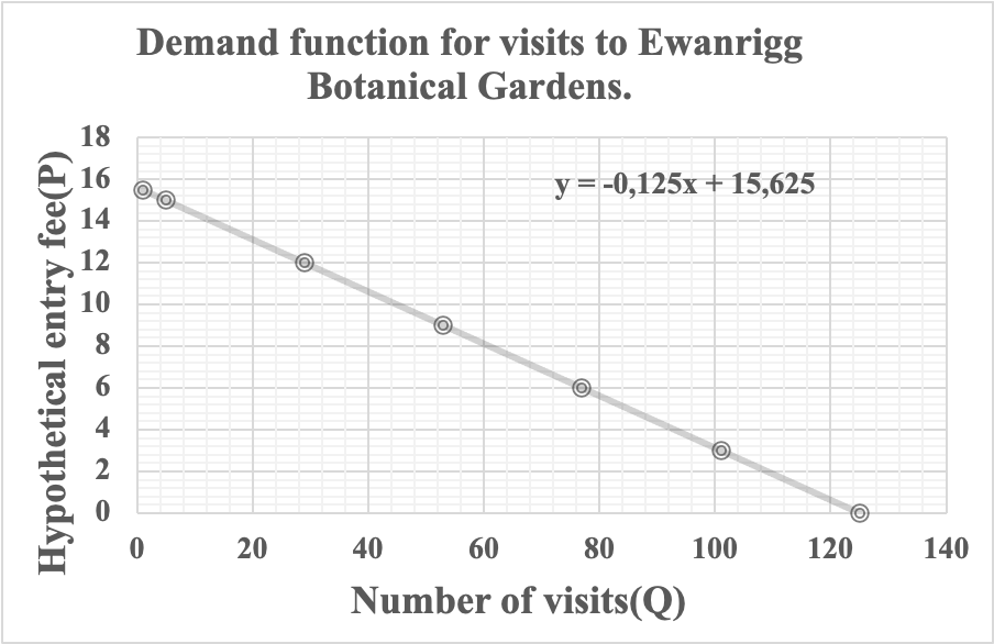
As shown in Fig 3, when P reached zero, Q was at a maximum (125 visitors) and when P was at a maximum the number of visits was zero (0). The demand equation was formulated as follows: P = -0.125Q + 15.625. Hence Q = 15.625÷ (2×0.125) = 62.5. Therefore P (optimum entrance fee) = (-0.125)62.5+15.625 = USD 7.81.
Conclusions and recommendations
This study aimed to estimate the imputed economic value of Ewanrigg Botanical Gardens in Zimbabwe using the Individual Travel Cost Method which elicits consumer surplus and deduce the entry fee. Comparable with major tourist destinations, travel costs, income and employment status were identified as the major factors through which visitation rates to Ewanrigg Botanical Gardens can be predicted. Using the Income Travel Cost Method the elicited economic value/peak period/year from recreational use of Ewanrigg Botanical Gardens was USD$19142.16. However, the research established that the current local visitor entry fee (USD3) to Ewanrigg Botanical Gardens was not optimal and was less than the estimated optimum entry fee of USD7.81.
It is imperative for the responsible authorities i.e. the Zimbabwe Parks and Wildlife Authorities to concentrate marketing efforts of Ewanrigg Botanical Gardens to groups of higher income and employment status as well as individuals within the proximity of the garden as these incur less travel costs. Furthermore, marketing should be done through a plethora of platforms such as billboards and electronic means (television, radio, online) which equally can attract potential male and female visitors. The central government through responsible line ministries should allocate adequate funds for management and or further development of Ewanrigg Botanical Gardens so as to attract more visitors from diverse socioeconomic backgrounds. A gradual increase in the optimum entrance fee to USD$7.81 will help maximize revenue for self-sustenance and continuity of Ewanrigg Botanical Gardens. On a regional and global scale it is imperative for responsible authorities to institute accurate economic valuation of the actual attraction site using formal means, and then afterwards value the ecosystem services and any other ancillary services. This will enable accurate estimation of the quantitative magnitude of ecosystem service benefits generated from public access.
Appendix
Appendix 1. Non-market valuation techniques

Appendix 2. Questionnaire used to solicit information on socioeconomic characteristics of visitors to Ewanrigg Botanical Gardens
This questionnaire was designed to obtain personal and socioeconomic information of visitors to Ewanrigg Botanical Gardens, Shamva, Zimbabwe. The survey was carried out by Kusuwo Kudakwashe Bryan in partial fulfilment of the requirements of the Bachelor of Science Honours degree in Environmental Science and Technology at Chinhoyi University of Technology. The obtained information were used for economic valuation of the garden only and did not discriminate any respondent. Feel free to answer the questions, your cooperation is greatly appreciated.
NB: Tick in the boxes ◻ and fill in your information in the spaces provided.
Personal information
1. Is Ewanrigg Botanical Gardens your final visit destination?
A. Yes ◻ A. No ◻
2. Place of residence? ………………………………………..
3. How did you get to Ewanrigg Botanical Gardens?
A.Road ◻ B.Walking ◻ C. Cycling ◻ D.Air E. Railway ◻
4. What is your purpose of visit?
A. Recreation ◻ B. Education ◻ C. Function ◻
5. How many times have you visited Ewanrigg Botanical Gardens in the last 12 months?
……………………………………….
Socioeconomic characteristics
6. Age …………….
7. Gender
A.Male ◻ B. Female ◻
8. Marital Status
A.Married ◻ B. Single ◻ C. Divorced ◻ D. Widowed ◻
9. Employment Status
A. Retired ◻ B. Student ◻ C.Unemployed ◻ D. Employed
10. Educational level
A. Primary ◻ B.Secondary ◻ C.Tertiary ◻
11. Monthly income
A.Less than $200 ◻ B. $200-500 ◻ C. $500-1000 ◻ D.above $1000 ◻
THANK YOU FOR YOUR TIME!
Appendix 3. Frequency tables of socioeconomic factors
| Travel Cost ($) | Frequency | Cumulative Frequency | Relative frequency |
| ≤11 | 25 | 20 | 46.3 |
| 11-13 | 20 | 45 | 37.0 |
| 13-15 | 5 | 50 | 9.3 |
| 15-17 | 3 | 53 | 5.6 |
| ≥17 | 1 | 54 | 1.9 |
| Educational Level (years) | Frequency of visitors | Cumulative frequency | Relative Frequency |
| Primary | 6 | 6 | 11.1 |
| Secondary | 11 | 17 | 20.4 |
| Tertiary | 37 | 54 | 68.5 |
| Age (years) | Number of visits | Cumulative frequency | Relative Frequency |
| 18-25 | 8 | 25 | 14.8 |
| 26-35 | 14 | 22 | 25.9 |
| 36-45 | 19 | 41 | 35.2 |
| 46-55 | 6 | 47 | 11.1 |
| 56-65 | 7 | 54 | 12.9 |
| Income groups | Number of visitors | Cumulative Frequency | Relative frequency (%) |
| Less than $200 | 5 | 2 | 9.3 |
| $200-500 | 16 | 21 | 29.7 |
| $500-1000 | 18 | 39 | 33.3 |
| 1000-1500 | 11 | 50 | 20.4 |
| >1500 | 4 | 54 | 7.4 |
| Marital Status | Frequency of visitors | Cumulative Frequency | Relative Frequency |
| Married | 30 | 30 | 55.6 |
| Single | 22 | 52 | 40.7 |
| Divorced | 0 | 52 | 0 |
| Widowed | 2 | 54 | 3.7 |
| Employment status | Frequency | Cumulative Frequency | Relative Frequency |
| Retired | 4 | 4 | 7.4 |
| Student | 5 | 9 | 9.3 |
| Unemployed | 8 | 17 | 14.8 |
| Employed | 37 | 54 | 68.5 |
| Gender | Frequency | Cumulative frequency | Relative frequency (%) |
| Male | 19 | 19 | 35.2 |
| Female | 35 | 54 | 64.8 |
Appendix 4. Results of linear regression analysis of the socioeconomic variables against the number of visits to EBG.
Travel Costs against number of visits of EBG
| Multiple R | 0,7652938 |
|---|---|
| R Square | 0,5856745 |
| Adjusted R Square | 0,5166203 |
| Standard Error | 18,107168 |
| Observations | 54 |
| df | SS | MS | F | Significance F | |
|---|---|---|---|---|---|
| Regression | 1 | 2780,7827 | 2780,7827 | 8,4813692 | 0,0269004 |
| Residual | 52 | 1967,2173 | 327,86955 | ||
| Total | 53 | 4748 |
| Coefficients | Standard Error | t Stat | P-value | Lower 95% | Upper 95% | Lower 95,0% | Upper 95,0% | |
|---|---|---|---|---|---|---|---|---|
| Intercept | 125,25285 | 35,352048 | 3,5430154 | 0,0121744 | 38,749506 | 211,7562 | 38,749506 | 211,7562 |
| Travel costs | -8,3662756 | 2,8727589 | -2,912279 | 0,0269004 | -15,395664 | -1,3368877 | -15,395664 | -1,3368877 |
Competing interests
The authors declare no conflict of interest whatsoever for this manuscript.
References
- Abercrombie, L. C., Sallis, J. F., Conway, T. L., Frank, L. D., Saelens, B. E., & Chapman, J. E. (2008). Income and racial disparities in access to public parks and private recreation facilities. American journal of preventive medicine, 34(1), 9-15.
- Agency, Z. N. S. (2012). Zimbabwe Population Census, 2012: Zimbabwe National Statistics Agency.
- Bartczak, A., Lindhjem, H., Navrud, S., Zandersen, M., & Żylicz, T. (2008). Valuing forest recreation on the national level in a transition economy: The case of Poland. Forest Policy and Economics, 10(7-8), 467-472.
- Bedate, A., Herrero, L. C., & Sanz, J. Á. (2004). Economic valuation of the cultural heritage: application to four case studies in Spain. Journal of Cultural Heritage, 5(1), 101-111.
- Bharali, A., & Mazumder, R. (2012). Application of travel cost method to assess the pricing policy of public parks: the case of Kaziranga National Park. Journal of Regional Development and Planning, 1(1), 44-52.
- Bishop, J., & Pagiola, S. (2012). Selling forest environmental services: market-based mechanisms for conservation and development: London. EarthScan.Taylor & Francis.
- Brander, L. M., & Koetse, M. J. (2011). The value of urban open space: Meta-analyses of contingent valuation and hedonic pricing results. Journal of environmental management, 92(10), 2763-2773.
- Carrus, G., Scopelliti, M., Lafortezza R., Colangelo G., Ferrini F., Salbitano, F., et al. (2015). Go greener, feel better? The positive effects of biodiversity on the well-being of individuals visiting urban and peri-urban green areas. Landscape. Urban Planning, 134, 221–228.
- Carpenter, S. R., Mooney, H. A., Agard, J., Capistrano, D., DeFries, R. S., Díaz, S., &Pereira, H. M. (2009). Science for managing ecosystem services: Beyond the Millennium Ecosystem Assessment. Proceedings of the National Academy of Sciences, pnas. 0808772106.
- Cesario, F. J. (1976). Value of time in recreation benefit studies. Land economics, 52(1), 32-41.
- Chacha, P., Muchapondwa, E., Wambugu, A., & Abala, D. (2013). Pricing of national park visits in Kenya: The case of Lake Nakuru National Park. Economic Research Southern Africa Working Paper, 357.
- Chae, D.-R., Wattage, P., & Pascoe, S. (2012). Recreational benefits from a marine protected area: A travel cost analysis of Lundy. Tourism Management, 33(4), 971-977.
- Chen, G., and Sun, W. (2018). The role of botanical gardens in scientific research, conservation, and citizen science. Plant Diversity, 40, 4: 181-188.
- Chikumbi, L. M. (2013). Optimal pricing for national park entrance fees in Zambia. University of Cape Town.
- Child, G. (2012). The emergency of modern nature conservation in Zimbabwe. Evolution and Innovation in Wildlife Conservation: Parks and Game Ranches to Transfrontier Conservation Areas, 67-84.
- Chung, J. Y., Kyle, G. T., Petrick, J. F., & Absher, J. D. (2011). Fairness of prices, user fee policy and willingness to pay among visitors to a national forest. Tourism Management, 32(5), 1038-1046.
- Clawson, M., & Knetsch, J. L. (2013). Economics of outdoor recreation: RFF Press.
- Costanza, R., de Groot, R., Sutton, P., Van der Ploeg, S., Anderson, S. J., Kubiszewski, I., & Turner, R. K. (2014). Changes in the global value of ecosystem services. Global environmental change, 26, 152-158.
- Das, S. (2013). Travel cost method for environmental valuation. Center of Excellence in Environmental Economics, Madras School of Economics, Dissemination Paper, 23.
- Davis, L. W. (2008). Durable goods and residential demand for energy and water: evidence from a field trial. The RAND Journal of Economics, 39(2), 530-546.
- Demir, A. (2014). Determination of the recreational value of botanic gardens. A case study royal botanic gardens, Kew, London. Revista de Cercetare si Interventie Sociala, 44, 160.
- Dixon, J., Scura, L., Carpenter, R., & Sherman, P. (2013). Economic analysis of environmental impacts: Routledge.pp 224.
- Draugalis, J. R., Coons, S. J., & Plaza, C. M. (2008). Best practices for survey research reports: a synopsis for authors and reviewers. American Journal of Pharmaceutical Education, 72(1), 11. doi: 10.5688/aj720111. PMID.
- Dumitraş, D. E., Felix, H., & Merce, E. (2011). A brief Economic Assessment on the Valuation of National and Natural Parks: the case of Romania. Notulae Botanicae Horti Agrobotanici Cluj-Napoca, 39(1), 134-138.
- Eker, Ö., & Demircioğlu, H. (2016). An application of travel-cost method and willingness to pay surveys for karatepe-aslantaş national park in Turkey. Aslantaş National Park in Turkey. 1st International Mediterranean Science and Engineering Congress, Çukurova University, Adana, Turkey, October 26-28, Çukurova University, 1316- 1321.
- Fernando, A.P.S., Nilushika, W.A.J, & Marasinghe, M.M.M.K. (2016). Recretional value of Muthurajawela ecosystem: An application of travel cost method. Journal of Agricultural Environmental Science, 24-32.
- Fleming, C. M., & Cook, A. (2008). The recreational value of Lake McKenzie, Fraser Island: An application of the travel cost method. Tourism Management, 29(6), 1197-1205.
- Freeman III, A. M., Herriges, J. A., & Kling, C. L. (2014). The measurement of environmental and resource values: theory and methods: 3 rd Edition. pp 478.Routledge.
- Ghimire, R., Green, G. T., Poudyal, N. C., & Cordell, H. K. (2014). An analysis of perceived constraints to outdoor recreation. Journal of Park and Recreation Administration, 32(4), 52-67.
- Gómez-Baggethun, E., De Groot, R., Lomas, P. L., & Montes, C. (2010). The history of ecosystem services in economic theory and practice: from early notions to markets and payment schemes. Ecological Economics, 69(6), 1209-1218.
- Grafton, R. Q., & Ward, M. B. (2008). Prices versus rationing: Marshallian surplus and mandatory water restrictions. Economic Record, 84, S57-S65.
- Golding, J., Güsewell, S, Kreft, H. et al. (2010). Species-richness patterns of the living collections of the world's botanic gardens: a matter of socio-economics? Annals of. Botany, 105, 689-696.
- Heesch, K. C., Giles-Corti, B., & Turrell, G. (2014). Cycling for transport and recreation: associations with socio-economic position, environmental perceptions, and psychological disposition. Preventive Medicine, 63, 29-35.
- Hill, J. L., & Gale, T. (2009). Ecotourism and environmental sustainability: principles and practice: Ashgate Publishing, Ltd.
- Iqbal, J., Khan, Y., Haq, Z., & Hesseln, H. (2017). Estimation of Economic Value of an Archaeological Site: A Case Study of Takht-i Bahi. Ancient Pakistan, 28, 85-95..
- Islam, K., & Majumder, S. (2015). Economic evaluation of Foy's lake, Chittagong using travel cost method. Indian Journal of Economics and Development, 3(8), 12-18.
- Jim, C., & Chen, W. Y. (2009). Value of scenic views: Hedonic assessment of private housing in Hong Kong. Landscape and Urban Planning, 91(4), 226-234.
- Jones, A., Wright, J., Bateman, I., & Schaafsma, M. (2010). Estimating arrival numbers for informal recreation: a geographical approach and case study of British woodlands. Sustainability, 2(2), 684-701.
- Kamphuis, C. B., Van Lenthe, F. J., Giskes, K., Huisman, M., Brug, J., & Mackenbach, J. P. (2009). Socioeconomic differences in lack of recreational walking among older adults: the role of neighbourhood and individual factors. International Journal of Behavioral Nutrition and Physical Activity, 6(1), 1.
- Kim, D.-H., Doyle, M. R., Sung, S., & Amasino, R. M. (2009). Vernalization: winter and the timing of flowering in plants. Annual Review of Cell and Developmental, 25, 277-299.
- Kothari, C. R. (2004). Research methodology: Methods and techniques: New Age International.
- Laarman, J. G., & Gregersen, H. M. (1996). Pricing policy in nature-based tourism. Tourism Management, 17(4), 247-254.
- Limaei, S. M., Ghesmati, H., Rashidi, R., & Yamini, N. (2014). Economic Evaluation of Natural Forest Park Using the Travel Cost Method (Case Study: Masouleh Forest Park, North of Iran)”. Journal of Forest Science, 60(6), 254-261.
- Manvitha, K., & Bidya, B. (2014). Aloe vera: a wonder plant its history, cultivation and medicinal uses. Journal of Pharmacognosy and Phytochemistry, 2(5), 85-88.
- Manzote, E. (2013). An application of the individual travel cost method to Nyanga National Park Zimbabwe.
- Martín-López, B., Gómez-Baggethun, E., Lomas, P. L., & Montes, C. (2009). Effects of spatial and temporal scales on cultural services valuation. Journal of environmental management, 90(2), 1050-1059.
- Martínez-Espiñeira, R., & Amoako-Tuffour, J. (2009). Multi-destination and multi-purpose trip effects in the analysis of the demand for trips to a remote recreational site. Environmental management, 43(6), 1146-1161.
- Moore, L. V., Roux, A. V. D., Evenson, K. R., McGinn, A. P., & Brines, S. J. (2008). Availability of recreational resources in minority and low socioeconomic status areas. American journal of preventive medicine, 34(1), 16-22.
- Mounce, R., Smith, P,. & Brockington, S. (2017). Ex situ conservation of plant diversity in the world's botanic gardens. Natural Plants, 3, 795-802.
- Mwebaze, P., & Bennett, J. (2012). Valuing Australian botanic collections: a combined travel‐cost and contingent valuation study. Australian Journal of Agricultural and Resource Economics, 56(4), 498-520.
- Ortaçeşme, V., Özkan, B., & Karagüzel, O. (2002). An estimation of the recreational use value of Kursunlu Waterfall Nature Park by the individual travel cost method. Turkish Journal of Agriculture and Forestry, 26(1), 57-62.
- Osunsina, I. (2017). Travel Cost Analysis of Tourist Visits to Okomu National Park, Nigeria. Nigerian Journal of Wildlife Management (NJWM), 1(1).
- Pak, M., & Türker, M. F. (2006). Estimation of recreational use value of forest resources by using individual travel cost and contingent valuation methods (Kayabaşı Forest Recreation site sample). Journal of Applied Sciences, 6(1), 1-5.
- Paracchini, M. L., Zulian, G., Kopperoinen, L., Maes, J., Schägner, J. P., Termansen, M., & Bidoglio, G. (2014). Mapping cultural ecosystem services: A framework to assess the potential for outdoor recreation across the EU. Ecological Indicators, 45, 371-385.
- Parsons, G. R. (2003). The travel cost model A primer on nonmarket valuation (pp. 269-329): Springer.
- Pojani, E. (2016). An economic valuation of tourism in Shëngjini Beach using the zonal travel cost method. 13 th International Conference of ASECU. Social and Economic Challenges in Europe
- Pratiwi, S. R. (2015). Economic valuation of Amal Beach tourism: Travel Cost Method (TCM) application. Conference: The 5th IRSA International Institute BaliAt: Denpasar.
- Ren, H and Duan, Z.Y. (2017). The Theory and Practice on Construction of Classic Botanical Garden Science Press, Beijing, China.
- Rolfe, J., & Dyack, B. (2010). Testing for convergent validity between travel cost and contingent valuation estimates of recreation values in the Coorong, Australia. Australian Journal of Agricultural and Resource Economics, 54(4), 583-599.
- Safitri, W. (2018). Valuasi ekonomi green tourism Pantai Lakey, kabupaten dompu: pendekatan metode biaya perjalanan.
- Sambury, C., Hutchinson, S., & Avril, D. H. (2011). Factors influencing the willingness to pay a user fee for a state forest recreation visitor facility. Paper presented at the 2011 West Indies Agricultural Economics Conference, July 17-21, 2011, St. Vincent, West Indies.
- Samdin, Z., Aziz, Y. A., Radam, A., & Yacob, M. R. (2010). Factors influencing the willingness to pay for entrance permit: The evidence from Taman Negara National Park. Journal of Sustainable Development, 3(3), 212‑217.
- Sander, H. A., & Haight, R. G. (2012). Estimating the economic value of cultural ecosystem services in an urbanizing area using hedonic pricing. Journal of environmental management, 113, 194-205.
- Sen, A., Harwood, A. R., Bateman, I. J., Munday, P., Crowe, A., Brander, L.,... Provins, A. (2014). Economic assessment of the recreational value of ecosystems: methodological development and national and local application. Environmental and Resource Economics, 57(2), 233-249.
- Shammin, M. R. (1999). Application of the travel cost method (TCM): a case study of environmental valuation of Dhaka Zoological garden. Published in “The Economic Value of the Environment: Cases from South Asia”, Kathmandu, Nepal, 39-56.
- Smith, V. K. (1989). Taking stock of progress with travel cost recreation demand methods: Theory and implementation. Marine resource economics, 6(4), 279-310.
- Stodolska, M., Shinew, K. J., Acevedo, J. C., & Roman, C. G. (2013). “I was born in the hood”: Fear of crime, outdoor recreation and physical activity among Mexican-American urban adolescents. Leisure Sciences, 35(1), 1-15.
- Tahzeeda, J., Khan, M. R., & Bashar, R. (2018). Valuation approaches to ecosystem goods and services for the National Botanical Garden, Bangladesh. Environmental & Socio-economic Studies, 6(1), 1-9.
- Tazkia, F. O., & Hayati, B. (2012). Analisis Permintaan Obyek Wisata Pemandian Air Panas Kalianget, Kabupaten Wonosobo Dengan Pendekatan Travel Cost. Fakultas Ekonomika dan Bisnis.
- Ten Brink, P. (2012). The economics of ecosystems and biodiversity in national and international policy making: Routledge.
- Tiwari, S., & Chatterje, S. (2017). Ecotourism in protected. Research Journal of Agriculture and Forest, 5(1), 1-6.
- Twerefou, D. K., & Ababio, D. K. A. (2012). An economic valuation of the Kakum National Park: An individual travel cost approach. African Journal of Environmental Science and Technology, 6(4), 23-32.
- Whitehead, J. C., Pattanayak, S. K., Van Houtven, G. L., & Gelso, B. R. (2008). Combining revealed and stated preference data to estimate the nonmarket value of ecological services: an assessment of the state of the science. Journal of Economic Surveys, 22(5), 872-908.
- Williams, S. J., Jones, J. P., Gibbons, J. M., & Clubbe, C. (2015). Botanic gardens can positively influence visitors’ environmental attitudes. Biodiversity and Conservation, 24(7), 1609-1620.
- Zandi, S., Limaei, S. M., & Amiri, N. (2018). An economic evaluation of a forest park using the individual travel cost method (a case study of Ghaleh Rudkhan forest park in northern Iran). Environmental & Socio-economic Studies, 6(2), 48-55.
- Zimbabwe Energy Regulatory Authority. (2017). Zimbabwe developing a vehicle fuel economy policy.Retrieved from www.greencarcongress.com/2017/12/20171229-zimbabwe.html.
- Zimbabwe Gasoline Prices. (2018). Retrieved from https://www.globalpetrolprices.com/Zimbabwe/gasoline_pries/
- Zimbabwe Parks and Wildlife Act. (2014).Retrieved from faolex.fao.org/docs/pdf/zim8942.
- Zimbabwe Parks and Wildlife Authority. (2017).Ewanrigg Botanical Gardens. Retrieved from zimparks.org/parks/botanic gardens/ewanrigg-botanical-gardens/.
- Zuze, S. (2013). Measuring the economic value of wetland ecosystem services in Malawi: A case study of Lake Chiuta wetland. Msc Thesis. University of Zimbabwe.
Open Peer Review
